How a Non-Mathematician Came to Understand Black-Scholes

In several of my previous posts I have mentioned (more accurately confessed and pleaded) that I am not a mathematician. In fact, as a young student I never went beyond advanced algebra in high school. Though I got a final grade of "A" in all my math classes (I did get a midterm grade of "C" in basic algebra), I was told by someone in authority that I did not have the ability for more advanced classes. Perhaps they were right. In any event, I never took a math class in college and always viewed mathematics as outside of my core competencies and strengths.

Much later in life, after I had finished careers in law and banking, I found myself teaching a class which I had developed entitled "Corporate Finance for Non-Finance Majors." At the very end were the materials for a class I sometimes chose to include depending on how the semester had gone. It was basically a very non-technical view of options. I explained what options were and how they worked — the inputs being strike price, interest rates, volatility and time to expiration. I showed my students the Black-Scholes option pricing formula, which is certainly one of the most extraordinary achievements in finance. I did some hand waving, told my students not to freak out and showed where each of the inputs could be found in the formula. And I made the point, which I thought important, that while in finance and investing volatility usually decreases value, in options it is the opposite. More volatility — more value. That was more than enough for non-finance students. And to be perfectly honest, it was pretty much all I was capable of doing.

But that bothered me — a lot. I wanted a better understanding, and I suppose I also wanted to fight back against the narrative that I just wasn't smart enough to figure it out. So, several years ago, with the encouragement of my sons and their wives — one of whom is a PhD mathematician — I started taking some online courses. First, statistics and then calculus. I spent innumerable hours (actually weeks) studying and going over materials. And then last summer I repeated the whole process over again — new courses that were more comprehensive and challenging.

And every once in a while, I would open up my computer and look at the Black-Scholes model for pricing options. Slowly, ever so slowly I came to believe that I could do this — understand this Noble Prize-winning achievement at a deep and intuitive level.

This article is my effort to share that journey with others who may also be interested.

Shock — OMG!! What the heck is going on?

When you first look carefully at the Black-Scholes formula the natural reaction — at least mine was — "What the hell is going on here? What are all these symbols? Forget it, I will never be able to make sense of any part of this?" But as panic and fear subside you begin to see a couple of things that perhaps make sense. Forget the definitions of N(d1) and N(d2). Look at just the basic equation:

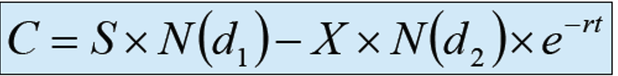
You see that according to the equation the value of a call option ("C") is equal to the price of the stock today ("S") multiplied by some funky term that might as well be Greek (together the "Stock Term"), minus the strike price of the option ("X") multiplied by even more ridiculous terms (together the "Option Term"). Okay, so that makes some sense. You know that at expiration the option is going to be worth the positive difference (if any) between S and X. If X is greater than S the option is worthless. So that feels good. You have taken one tiny baby step, and you haven't immediately fallen on your face. So you keep going.

Next, you notice that the Stock Term and the Option Term have a lot in common. Both involve multiplying by "N", which is the Cumulative Density Function of a Standard Normal Distribution (a mouthful that I have written about elsewhere). The first is obtained by multiplying by N(d1) and the second by N(d2). Besides (d1) and (d2) obviously being different (you will need to face that at some point) the Option Term is also multiplied by e^−rt. What is that all about? You rack your brain and finally remember that the term is the formula for the continuously discounted present value with "r" representing the discount rate, "t" the time stated in years and "e" that almost magical Euler's number. So, you are discounting the Option Term to determine its present value but not discounting the Stock term. Hmmm? How do I think about that?

This is the first point at which you find yourself in an intellectual struggle and at risk of losing everything. But wait a minute! The Stock Term incorporates the price of the stock today while the Option Term refers to a strike price that will only be paid, if ever, at expiry of the option at some point in the future. It makes total sense to discount the latter but not the former. Crisis avoided. Now what?

The next thing you notice, (and in the end, this is going to be the source of so much confusion) is that the definitions of N(d1) and N(d2) share a lot in common. In fact, N(d2) is just a particular adjusted form of N(d1):

It may take several minutes, or hours or a long walk outside (I try to walk 4–5 miles every day) before your stomach settles down but at some point, you are able to think clearly enough to observe that both terms contain symbols ordinarily associated with probability theory. The first term (d1) contains both variance ("σ²") and standard deviation ("σ") and the second term (d2) contains the symbol for standard deviation. So, now you are beginning to make real progress.

At this point, everything seems to click into place. You see variance. You see standard deviation. You see what looks like a normal distribution. And you think: Of course, this must be about probabilities. We are trying to figure out the likelihood that, at expiration, the stock price will be above the strike price. That will determine whether the option will actually be worth anything. That feels right. More than right — it feels obvious.

Unfortunately, if you follow your intuition here and go down the road of thinking that Black-Scholes is all about determining probabilities you are headed down a road that will take you into a forest (perhaps better described as a jungle) from which you will never emerge. You might as well sit down and cry. You are NOT getting out! I went down this road and while I didn't end up crying, I found myself lost, doubting my own intelligence and thinking that mathematicians must be some special species of human that have as much in common with me as a human does with an amoeba.

It is true that there is some concept of probability built into the Black-Scholes formula — particularly the Option Term — and we will get to that in due course. But the essential thing you need to understand — really understand — is this:

It is about constructing a portfolio — using stock and borrowed money — that will produce exactly the same payoff as the option.

Here is something worth keeping in mind. If you want to acquire something that will give you the same payout as the option, of course you can buy the option. Unfortunately, that doesn't do much to help you figure out its value. To do that, you need to create the identical payoff with things that have market value independent of what you are trying to do. Those things happen to be the stock involved and leverage — or borrowed funds.

And let me offer two insights that helped me a lot. First, if you buy some amount of stock, finance it with some amount of debt, and let it sit you are not going to end up where you would be at expiry if you owned the option. Why? Because the payoff depends upon the relationship between the stock price and the strike price at expiry. And while the strike price is fixed, the stock price obviously isn't. If it were, there would be nothing to option. Second, and this is a bit of a reiteration of what I said above, if you look closely at the Black Scholes formula you will notice, in addition to a lot of symbols that you may not understand — that the formula, stripped of all those symbols — is basically the value of the stock minus the strike price. Everything else is just an adjustment to one of these two values intended to take care of volatility (uncertainty), time to expiration, and interest rates. The incredible thing is that these two terms, obvious in one respect, take on additional meanings that seem either magical or one extraordinary coincidence. Let's find out.

Where to start — N(d1) or N(d2)?

Almost all discussions and presentations I have come across on Black-Scholes begin with an analysis of N(d2). It is generally assumed that from a conceptual viewpoint this is the simpler of the two (notwithstanding that it is derived from N(d1) — go figure). However, what I discovered after hours and hours of focus and a bit of screaming and table pounding is that at least for me this was the wrong way around. It is ironic, but I found that if you tackle N(d2) first and understand it — really understand it, internalize it — it is exceedingly difficult and unnecessarily hard to think correctly about N(d1). But enough generalities and warnings.

I suppose there are two basic approaches to wrestling N(d1) to the ground. One way to approach N(d1) is to dissect every symbol and every term and then try to figure out what N(d1) is intended to achieve by reference to its components. To do this, I think you really do need to be a mathematician and a hell of a good one. I tried that approach. For me, it was a disaster. All I achieved was a headache and a feeling of total incompetence.

So, I changed the question. I stopped wondering what all the symbols and terms meant. Instead, I asked: What problem is N(d1) solving? This change led to a major breakthrough. If Black-Scholes is fundamentally about replication, then the first question I need to answer is simple: How much stock do I need to hold in the replicating portfolio? That, as I slowly came to understand, is what N(d1) is doing.

Let's start with a couple of very simple insights:

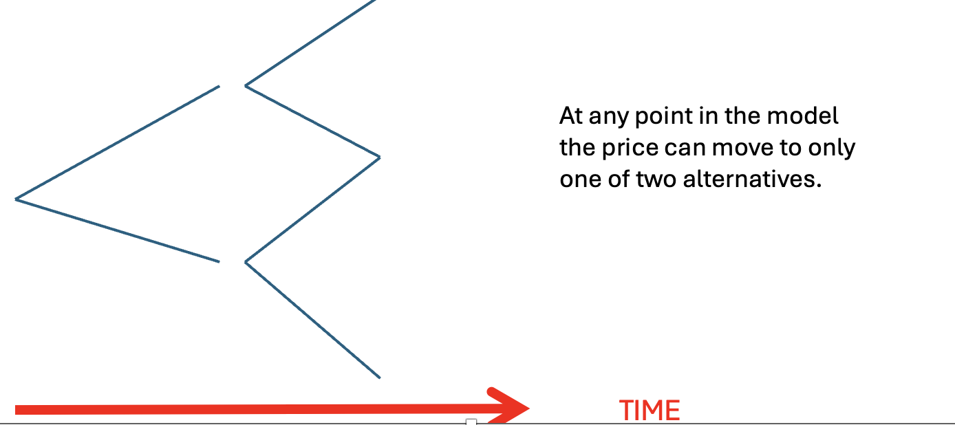
POINT ONE: The Black-Scholes model is just a special case (albeit a complicated one) of a binomial option pricing model.

POINT TWO: If we can create a package of assets, each with a clearly ascertainable cost (referred to as the replicating portfolio), that generate the same cash flows as the option we are trying to analyze, we can assume that the option must have the same value as the package of assets. Why? Because otherwise the market could arbitrage the two and generate a riskless return, i.e., free money (sometimes called a "free lunch).

To get a handle on this we are going to create a simple replicating portfolio by using a combination of:

1. Underlying stock; and
2. Borrowing.

By building the portfolio and applying the concept of "no arbitrage" we will be able to derive the value of a simple call option using a binomial option pricing strategy over one period.

This is easy!!

Assume you are looking at stock that is currently trading at $100 per share. You are considering a call option with a one-year expiration and a strike price of $100. Interest rates are 5%. A year from now the stock will either be at $90 per share or $110. So, at expiry the option will either be worth $10 or nothing. How do I determine the value of the option? I can ask a relatively simple question: How much stock do I need to buy today, and how much money do I need to borrow, to create those exact same outcomes? To avoid the possibility of arbitrage the cost of doing that must be equal to the value of the option.

You may need to dust off the cobwebs in your mind but, alas, this is nothing but high school math! Two equations and two variables.

The critical insight here is not the arithmetic itself, but what it tells us: the option can be replicated by holding half a share of stock (cost $50) and financing part of that purchase ($42.86) with borrowed money. That must be the value of the option today: $7.14.

In Black-Scholes, the exact same questions exist: How many shares do we need now? How much do we borrow? The answer to that first question — the stock component of the hedge — is N(d1). It is going to get more complicated and a lot more confusing. But if you anchor your thinking in this basic understanding of what you are trying to accomplish you have the compass necessary to navigate your way through.

From One Period Binomial to Black-Scholes

You don't have to be a genius or anything approaching one to see right away that the Black-Scholes model is a whole lot more complex than the simple, one-period binomial model. For starters, Black-Scholes is generally dealing with multiple time periods and multiple, cumulative outcomes. Perhaps even more importantly, the binomial model assumed that the stock price would end up in only one of two places. Black-Scholes, on the other hand, needs to take account of essentially an unlimited number of possible outcomes. This is captured by building into the formula the Cumulative Distribution Function of the Standard Normal Distribution.

N(d1) as a Dynamic Hedge Ratio

Another obvious difference between the binomial model and Black-Scholes is that the former is a one-time, single point in time calculation. But, of course, stock markets are not fixed, and stock prices move continuously. Therefore, the replicating portfolio will be constantly in flux reflecting the changing stock price and other factors we will get to later. So, Black-Scholes is calculating a dynamic hedge ratio or what the replicating portfolio has to be moment to moment. It helps to keep this in mind — I certainly found this an important concept.

One Crucial Insight Before Digging Into N(d1)

There is one fundamental point that deserves reiteration before moving on. If you were approaching Black-Scholes completely anew, you might well think that pricing an option requires predicting the future. In the usual investing mindset, you focus on a stock's expected return which (often in unpredictable ways) takes account of macro factors, market dynamics and company factors such as profitability, cost structure, competitive advantages, strength of management and a host of other company-specific factors (sometimes referred to as idiosyncratic risk).

But according to Black-Scholes none of that is required to price an option. And that is truly the extraordinary part. To price an option, we only need to hedge dynamically the position using a combination of the underlying stock and borrowed money. That's it! Expected returns on the stock are irrelevant. Investor preferences regarding risk and return are irrelevant. "Views" on the stock, whether from professional traders, chartists, long-term fundamental investors, academics or retail investors are all irrelevant. Wow! This is something special.

Let's Understand N(d1)

We now know what question N(d1) is answering. It is answering the same question we answered in the one-period binomial world: How much stock do I need to hold right now so that my portfolio moves like the option? The only difference is that in Black-Scholes the answer changes continuously as the stock price, as well as other factors change. That is what makes N(d1) so extraordinary.

If N(d1) is the stock component of the hedge, then what should determine its size? I found it helpful to ask what the hedge ratio should look like in obvious situations. If the option is deep in the money and there is almost no time left, it should behave almost exactly like the stock. In that case, the hedge ratio should be very close to 1. On the other hand, if the option is far out of the money and close to expiry, it barely reacts to the stock at all. There, the hedge ratio should be close to 0. So whatever the hedge ratio is, it must give us a number that moves smoothly between 0 and 1, depending on how "alive" the option still is. That number is exactly N(d1).

With this insight it is actually not too difficult to develop a list of factors that would be relevant to determining the hedge ratio: (1) how close the stock is to the strike; (2) how much time remains before expiry of the option; (3) how volatile the stock is; and (4) interest rates. After pounding all of this into my head I was finally ready to look directly at the formula for d1, not as a jungle of symbols, but as a compact way of expressing everything I already knew must matter.

My Conceptual Breakthrough

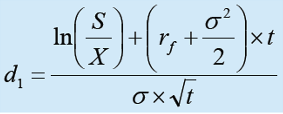
It should surprise no one that I struggled for a very long time with this very intimidating formula. There were more than a few moments when I said to myself "Screw it! I should focus on something else or go to the gym." But then I had a thought. I realized I was making it harder than it needed to be. The formula becomes far more intuitive if you think of it as two separate ideas sharing the same denominator.

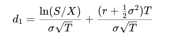
While at first this may seem to be making matters worse, it actually provided me with a huge intellectual breakthrough and the ability to ask two distinct questions:

Where is the stock relative to the strike right now? This is the first term.

How should that position be adjusted for time, interest rates, and volatility? This is the second term. Once I broke the formula apart this way, it stopped feeling like advanced mathematics and more like common sense written compactly.

Distance between Current Stock Price and the Strike Price

I got hung up here because the expression ln(S/X) looks almost exactly like the continuously compounded rate of return formula I had studied and even taught before. But then I realized something important. In Black-Scholes we are not measuring a return through time. We are measuring the relative distance between where the stock is today and where it needs to be for the option to get exercised. And that is captured by ln(S/X).

Why use logs? The log simply converts that distance into a percentage term rather than a dollar term. That matters because $10 means different things at different stock levels, while 10% means the same proportional distance. A simple example:

• $100 vs $110 = 10%
• $20 vs $30 = 50%

The option only "cares" about the relative hurdle, not raw dollars. In other words, ln(S/X) is Black-Scholes' way of asking: How far above or below the strike are we right now, in proportional terms? And the denominator makes perfect sense — we want to measure that distance in units of expected uncertainty, or how far the stock price is from the strike in terms of the amount the stock is expected to "wiggle" over the remaining life of the option. That is captured by the denominator σ√T.

What took me a little longer was understanding why time appears as the square root of T rather than just T. The answer is that uncertainty does grow as time passes, but not in a simple linear way. If you double the time horizon, you do not double the standard deviation of possible outcomes. Instead, what doubles is the variance, and standard deviation is simply the square root of variance. That is why the adjustment happens through √T.

Of course, there are several factors that determine the stock portion of the hedge. In addition to the distance between the stock today and the strike we need to take account of prevailing interest rates; the time left to expiry; and the volatility of the stock. This is exactly what the second term is designed to measure:

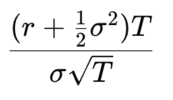
The term r stands for the risk-free rate. Once the stock and borrowing positions are combined to eliminate risk, the resulting portfolio cannot be expected to earn anything other than the risk-free rate. In the Black-Scholes model, this is not because the real world is assumed to be risk-neutral. Rather, Black-Scholes constructs a pricing world in which assets are assumed to grow at the risk-free rate because that is the world in which arbitrage disappears and the option can be priced by replication rather than prediction.

That is what makes the assumption so useful. It allows us to stop worrying about what investors believe, what return they demand, or whether the stock is "really" expected to outperform or underperform. Once replication and no-arbitrage do their work, those questions fall away.

This leaves one last term:

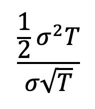
And this, at least for me, was the toughest part to absorb. Volatility does not simply make outcomes more spread out. In the Black-Scholes world, prices are assumed to be lognormally distributed, which means the distribution is not symmetric. It is skewed to the right. Prices cannot go below zero, but they can rise a great deal. Because of that asymmetry, volatility does more than add uncertainty. It also affects where the center of future outcomes effectively sits.

That is what this term is correcting for. It is the model's way of recognizing that once prices are lognormal, more volatility changes not only the width of possible outcomes, but also the weighting of the upside. And, of course, we standardize all of this in terms of units of expected uncertainty by dividing by σ√T.

Once I saw all of this, d1 no longer looked like an arbitrary mathematical construction. It looked like exactly what it was: a compact way of expressing the current position of the stock relative to the strike, adjusted for time, rates, volatility, and all measured in units of expected uncertainty. What had once looked like a jungle of symbols now felt almost inevitable. For the first time, I saw not just logic, but beauty.

The Mind-Blowing Coincidence That Is Not a Coincidence — N(d2)

If you are speaking with a group of folks about N(d2) you will likely hear a bunch of people describe N(d2) as the amount of money that needs to be borrowed as part of the hedging strategy. Others will say that it represents the likelihood that the stock price will be above the strike at expiry and therefore that the option will get exercised. The incredible truth is that both explanations are correct! As impossible as this may seem (and it seemed to me at first totally ridiculous), the same term that helps determine how much money we effectively borrow today also turns around and tells us the likelihood that the option will actually be exercised.

The answer, I slowly realized, is that the correct focus is not whether the debt itself is disappearing. Of course it's not. In the out-of-the-money states, the stock side of the hedge simply covers the debt repayment and leaves nothing extra, which is exactly what the option is worth there: zero. What matters is not whether the debt exists, but when the strike-side of the payoff contributes positive economic value to the option. That only happens in the states where the option finishes in the money. Put a slightly different way, the same probability distribution curve of future-states determines where the strike affects payoff and where the option is exercised. Those are literally the same set of states. Therefore, the same weighting object appears.

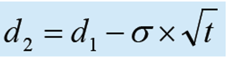
The incredible and double mind-blowing fact is that d2 is defined in terms of d1 and is actually remarkably close:

d2 = d1 − σ√T

And here is the deepest beauty of all: N(d1) and N(d2) are the same cumulative normal distribution calculation separated by exactly σ√T, which is the stock's expected standard deviation over the remaining life of the option. That exact shift captures the difference between two related but distinct questions: how strongly the option behaves like the stock today, and whether the stock merely finishes above the strike at expiry. That is why they are so closely related.

N(d1) gives weight to how far above the strike the stock might end up, because the stock side of the hedge must respond to the potential size of in-the-money outcomes. N(d2), by contrast, only asks whether the stock ends up above the strike at all.

What stunned me in the end was not merely that the same model could tell us how much stock to hold, how much money to borrow, and the likelihood of exercise. It was that all three emerged from nearly the same mathematical calculation. The hedge ratio, the borrowing term, and the probability of exercise are not separate ideas awkwardly stitched together. They are different economic interpretations of the same underlying future distribution of stock prices. What had first looked like a jungle of symbols had resolved itself into one coherent idea.

None of this, of course, means that real-world stock returns obediently follow a perfect lognormal distribution. Models are not valuable because reality conforms perfectly to them. They are valuable because they illuminate structure, relationships, and ways of thinking. Understanding the internal elegance of Black-Scholes is, at least to me, worthwhile even while fully recognizing where real markets depart from its assumptions.

My Journey

This has been a long journey but a very intellectually and emotionally satisfying one. In one respect it began months or even years ago when I embarked on an expedition to explore the mathematical underpinnings of finance. But if I am honest with myself, this journey began back in what was then called junior high school. I was told that I didn't have the intellectual capacity for any type of advanced mathematics or that the amount of effort I would need to put into it would be too much. I believed what I was told. Why wouldn't I? And so, I steered away from anything mathematical, never even pursuing mathematics in college.

However, it is hard to predict where life will take you and an early professional career in the law led to a longer career in banking and finance and ultimately teaching. I started wondering about all sort of things mathematical — taking online courses in statistics and calculus. The more I learned the more I wanted to know. There was Euler's number; the normal (Gaussian) curve; and always in the background that incredibly intimidating Black-Scholes option pricing formula.

I knew that at some point I would have to face all the symbols in that model. When I finally felt I was ready, I started very tentatively researching. I spent perhaps a ridiculous amount of time thinking about this. Sometimes I woke up in the middle of the night thinking about Black-Scholes. None of it made a whole lot of sense until I came to understand that notwithstanding appearances and what seemed obvious, Black-Scholes was first and foremost about replicating, hedging and no arbitrage and that probabilities played an important but supporting role. From that singular insight the entire structure started to reveal itself.

At some point I learned that there is an entirely different and much more formal route into Black-Scholes through partial differential equations ("PDEs"). I am grateful I did not start there or try to pursue that line of inquiry. It opens the door to an entirely different way of thinking about options through sensitivities — the Greeks: Delta, Gamma, Vega, Theta, and Rho. Those are best left to option traders. For the journey I needed to take, at this point in my life, replication and economic intuition were the only path that ever had a chance of working.

In the end, this journey was about far more than an option pricing formula. It was about discovering that understanding does not belong exclusively to specialists, and that what once appears impenetrable can give way, slowly and sometimes painfully, to persistence, curiosity, and the willingness to keep asking better questions. This last point was crucial. What I lacked in mathematical experience and formal training I made up for with the most rigorous thinking I could manage. I worked hard to make sure every single dot was connected. I fought against hand waving even from experts.

This journey through Black-Scholes gave me something I never expected: not just intuition and understanding but a renewed sense that the boundaries of our understanding are often far wider than the stories we inherit about ourselves. In my personal case the journey gave me a very much needed and desired new perspective of my own capabilities.